ANALISIS PENJUALAN TOKO RETAIL#
import pandas as pd
import matplotlib.pyplot as plt
df = pd.read_csv('retail_sales_dataset.csv')
df.head()
| Transaction ID | Date | Customer ID | Gender | Age | Product Category | Quantity | Price per Unit | Total Amount | |
|---|---|---|---|---|---|---|---|---|---|
| 0 | 1 | 2023-11-24 | CUST001 | Male | 34 | Beauty | 3 | 50 | 150 |
| 1 | 2 | 2023-02-27 | CUST002 | Female | 26 | Clothing | 2 | 500 | 1000 |
| 2 | 3 | 2023-01-13 | CUST003 | Male | 50 | Electronics | 1 | 30 | 30 |
| 3 | 4 | 2023-05-21 | CUST004 | Male | 37 | Clothing | 1 | 500 | 500 |
| 4 | 5 | 2023-05-06 | CUST005 | Male | 30 | Beauty | 2 | 50 | 100 |
df.describe()
| Transaction ID | Age | Quantity | Price per Unit | Total Amount | |
|---|---|---|---|---|---|
| count | 1000.000000 | 1000.00000 | 1000.000000 | 1000.000000 | 1000.000000 |
| mean | 500.500000 | 41.39200 | 2.514000 | 179.890000 | 456.000000 |
| std | 288.819436 | 13.68143 | 1.132734 | 189.681356 | 559.997632 |
| min | 1.000000 | 18.00000 | 1.000000 | 25.000000 | 25.000000 |
| 25% | 250.750000 | 29.00000 | 1.000000 | 30.000000 | 60.000000 |
| 50% | 500.500000 | 42.00000 | 3.000000 | 50.000000 | 135.000000 |
| 75% | 750.250000 | 53.00000 | 4.000000 | 300.000000 | 900.000000 |
| max | 1000.000000 | 64.00000 | 4.000000 | 500.000000 | 2000.000000 |
df.info()
<class 'pandas.core.frame.DataFrame'>
RangeIndex: 1000 entries, 0 to 999
Data columns (total 9 columns):
 #   Column            Non-Null Count  Dtype
---  ------            --------------  -----
 0   Transaction ID    1000 non-null   int64
 1   Date              1000 non-null   object
 2   Customer ID       1000 non-null   object
 3   Gender            1000 non-null   object
 4   Age               1000 non-null   int64
 5   Product Category  1000 non-null   object
 6   Quantity          1000 non-null   int64
 7   Price per Unit    1000 non-null   int64
 8   Total Amount      1000 non-null   int64
dtypes: int64(5), object(4)
memory usage: 70.4+ KB
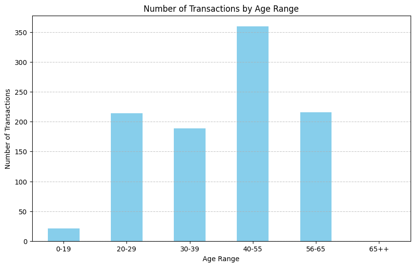
dari sini kita bisa mengetahui rentan usia terbanyak membeli adalah usia 40-55
bins = [0, 19, 29, 39, 55, 65, float('inf')]
labels = ['0-19', '20-29', '30-39', '40-55', '56-65', '65++']

# Add a new column for age range
df['Age Range'] = pd.cut(df['Age'], bins=bins, labels=labels, right=False)

# Count the number of transactions for each age range
age_range_counts = df['Age Range'].value_counts().sort_index()

# Plotting the data
plt.figure(figsize=(10, 6))
age_range_counts.plot(kind='bar', color='skyblue')
plt.title('Number of Transactions by Age Range')
plt.xlabel('Age Range')
plt.ylabel('Number of Transactions')
plt.xticks(rotation=0)
plt.grid(axis='y', linestyle='--', alpha=0.7)
plt.show()
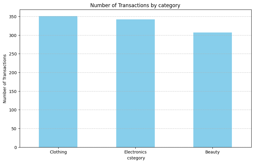
dapat kita ketahui kategori terlaris adalah clothing dengan jumlah pembelian 350 barang
# Menghitung jumlah transaksi untuk setiap gender
category_counts = df['Product Category'].value_counts()

# Plotting the data
plt.figure(figsize=(10, 6))
category_counts.plot(kind='bar', color='skyblue')
plt.title('Number of Transactions by category')
plt.xlabel(' cstegory')
plt.ylabel('Number of Transactions')
plt.xticks(rotation=0)
plt.grid(axis='y', linestyle='--', alpha=0.7)
plt.show()
#
# Menghitung jumlah transaksi untuk setiap gender
gender_counts = df['Gender'].value_counts()
# Plotting the data
plt.figure(figsize=(10, 6))
gender_counts.plot(kind='bar', color='skyblue')
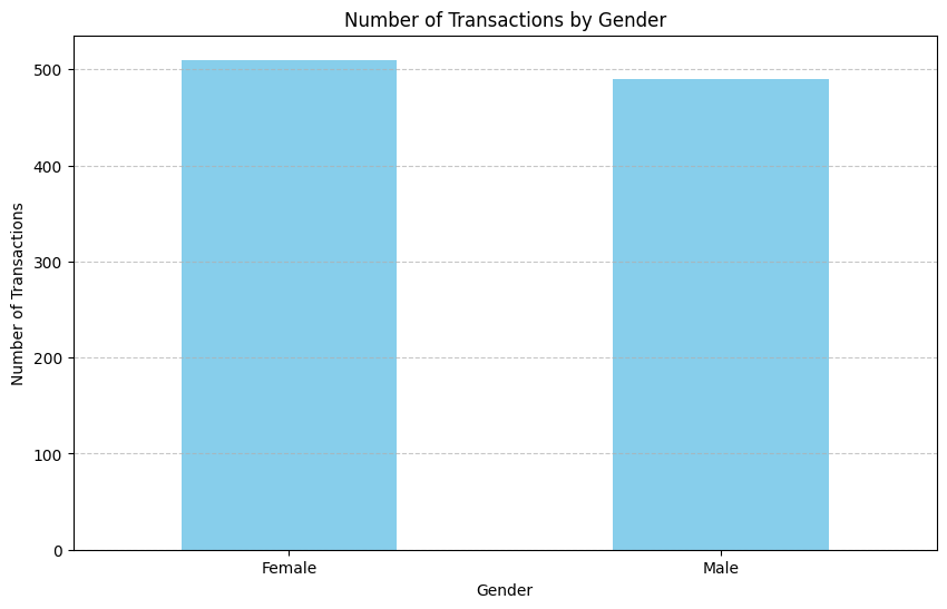
plt.title('Number of Transactions by Gender')
plt.xlabel('Gender')
plt.ylabel('Number of Transactions')
plt.xticks(rotation=0)
plt.grid(axis='y', linestyle='--', alpha=0.7)
plt.show()
# Menghitung jumlah transaksi untuk setiap kombinasi gender dan kategori produk
product_counts_by_gender = df.groupby(['Gender', 'Product Category']).size().unstack().fillna(0)
# Menampilkan hasil
print(product_counts_by_gender)
# Plotting the product counts by gender
product_counts_by_gender.plot(kind='bar', stacked=True, figsize=(12, 7), color=['skyblue', 'lightgreen', 'lightcoral', 'orange', 'purple'])
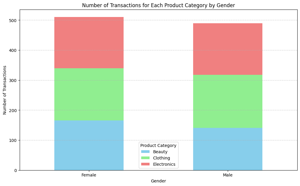
plt.title('Number of Transactions for Each Product Category by Gender')
plt.xlabel('Gender')
plt.ylabel('Number of Transactions')
plt.xticks(rotation=0)
plt.legend(title='Product Category')
plt.grid(axis='y', linestyle='--', alpha=0.7)
plt.show()
Product Category  Beauty  Clothing  Electronics
Gender
Female               166       174          170
Male                 141       177          172
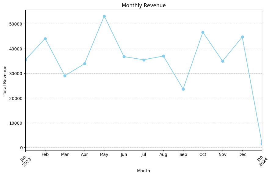
berikut adalah grafik pendapatan stiap bulan pendapatan tertinggiterdapat pada bulan mei dengan pendapatan total 53.150$
# Mengubah kolom 'Date' menjadi tipe data datetime
df['Date'] = pd.to_datetime(df['Date'])

# Menambahkan kolom 'Month' untuk bulan dan tahun
df['Month'] = df['Date'].dt.to_period('M')

# Menghitung total pendapatan untuk setiap bulan
monthly_revenue = df.groupby('Month')['Total Amount'].sum()

# Menampilkan hasil
print(monthly_revenue)

# Plotting the monthly revenue using a line plot
plt.figure(figsize=(10, 6))
monthly_revenue.plot(kind='line', marker='o', color='skyblue')
plt.title('Monthly Revenue')
plt.xlabel('Month')
plt.ylabel('Total Revenue')
plt.xticks(rotation=45)
plt.grid(axis='y', linestyle='--', alpha=0.7)
plt.show()
Month
2023-01    35450
2023-02    44060
2023-03    28990
2023-04    33870
2023-05    53150
2023-06    36715
2023-07    35465
2023-08    36960
2023-09    23620
2023-10    46580
2023-11    34920
2023-12    44690
2024-01     1530
Freq: M, Name: Total Amount, dtype: int64
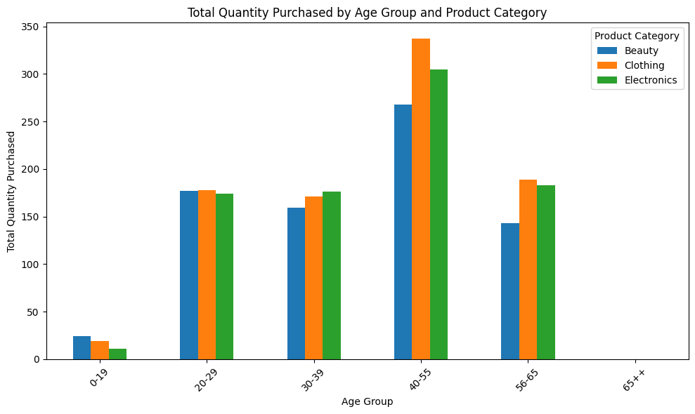
berikut adalah rentang usia dengan pemebelian kategori barang terbanyak ,seperti yang saya jelaskan di atas pembelian terbanyak terdapat pada usia 40-55 dengan rincian total pembelian clothing 337 , beauty 268, electronics 305
df['Age Group'] = pd.cut(df['Age'], bins=bins, labels=labels, right=False)

# Menghitung jumlah total pembelian untuk setiap kelompok kategori produk dan rentang usia
grouped_data = df.groupby(['Product Category', 'Age Group'])['Quantity'].sum().reset_index()

print(grouped_data)

# Membuat plot
fig, ax = plt.subplots(figsize=(10, 6))
grouped_data.pivot(index='Age Group', columns='Product Category', values='Quantity').plot(kind='bar', ax=ax)
plt.title('Total Quantity Purchased by Age Group and Product Category')
plt.xlabel('Age Group')
plt.ylabel('Total Quantity Purchased')
plt.xticks(rotation=45)
plt.tight_layout()
plt.show()
   Product Category Age Group  Quantity
0            Beauty      0-19        24
1            Beauty     20-29       177
2            Beauty     30-39       159
3            Beauty     40-55       268
4            Beauty     56-65       143
5            Beauty      65++         0
6          Clothing      0-19        19
7          Clothing     20-29       178
8          Clothing     30-39       171
9          Clothing     40-55       337
10         Clothing     56-65       189
11         Clothing      65++         0
12      Electronics      0-19        11
13      Electronics     20-29       174
14      Electronics     30-39       176
15      Electronics     40-55       305
16      Electronics     56-65       183
17      Electronics      65++         0
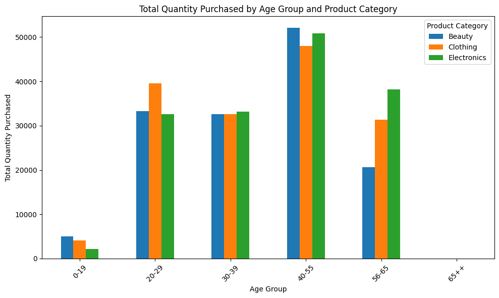
berikut adalah rentang usia dengan pengeluaran terbanyak ,seperti yang saya jelaskan di atas pembelian terbanyak terdapat pada usia 40-55 dengan rincian beauty 52.080 dolar, clothing 48015 dolar, electronics 50830
df['Age Group'] = pd.cut(df['Age'], bins=bins, labels=labels, right=False)

# Menghitung jumlah total pembelian untuk setiap kelompok kategori produk dan rentang usia
grouped_data_amount = df.groupby(['Product Category', 'Age Group'])['Total Amount'].sum().reset_index()
print(grouped_data_amount)

# Membuat plot
fig, ax = plt.subplots(figsize=(10, 6))
grouped_data_amount.pivot(index='Age Group', columns='Product Category', values='Total Amount').plot(kind='bar', ax=ax)
plt.title('Total Quantity Purchased by Age Group and Product Category')
plt.xlabel('Age Group')
plt.ylabel('Total Quantity Purchased')
plt.xticks(rotation=45)
plt.tight_layout()
plt.show()
   Product Category Age Group  Total Amount
0            Beauty      0-19          4960
1            Beauty     20-29         33250
2            Beauty     30-39         32555
3            Beauty     40-55         52080
4            Beauty     56-65         20670
5            Beauty      65++             0
6          Clothing      0-19          4085
7          Clothing     20-29         39565
8          Clothing     30-39         32605
9          Clothing     40-55         48015
10         Clothing     56-65         31310
11         Clothing      65++             0
12      Electronics      0-19          2170
13      Electronics     20-29         32555
14      Electronics     30-39         33140
15      Electronics     40-55         50830
16      Electronics     56-65         38210
17      Electronics      65++             0
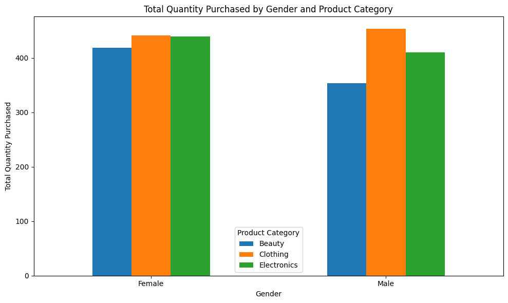
berikut adalah jumlah barang yang di beli olaeh setiap gender dengan rincian Beauty Female 418 Beauty Male 353 Clothing Female 441 Clothing Male 453 Electronics Female 439 Electronics Male 410
# Mengelompokkan data berdasarkan kategori produk dan jenis kelamin
grouped_gender_data = df.groupby(['Product Category', 'Gender'])['Quantity'].sum().reset_index()

print(grouped_gender_data)

# Membuat plot
fig, ax = plt.subplots(figsize=(10, 6))
grouped_gender_data.pivot(index='Gender', columns='Product Category', values='Quantity').plot(kind='bar', ax=ax)
plt.title('Total Quantity Purchased by Gender and Product Category')
plt.xlabel('Gender')
plt.ylabel('Total Quantity Purchased')
plt.xticks(rotation=0)
plt.tight_layout()
plt.show()
  Product Category  Gender  Quantity
0           Beauty  Female       418
1           Beauty    Male       353
2         Clothing  Female       441
3         Clothing    Male       453
4      Electronics  Female       439
5      Electronics    Male       410
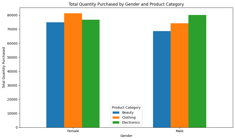
berikut adalah jumlah pengeluaran yang dikeluarkan oleh setiap gender dengan rincian Product Category Gender Total Amount Beauty Female 74830 Beauty Male 68685 Clothing Female 81275 Clothing Male 74305 Electronics Female 76735 Electronics Male 80170
# Mengelompokkan data berdasarkan kategori produk dan jenis kelamin
grouped_gender_data_bayar = df.groupby(['Product Category', 'Gender'])['Total Amount'].sum().reset_index()
print(grouped_gender_data_bayar)

# Membuat plot
fig, ax = plt.subplots(figsize=(10, 6))
grouped_gender_data_bayar.pivot(index='Gender', columns='Product Category', values='Total Amount').plot(kind='bar', ax=ax)
plt.title('Total Quantity Purchased by Gender and Product Category')
plt.xlabel('Gender')
plt.ylabel('Total Quantity Purchased')
plt.xticks(rotation=0)
plt.tight_layout()
plt.show()
  Product Category  Gender  Total Amount
0           Beauty  Female         74830
1           Beauty    Male         68685
2         Clothing  Female         81275
3         Clothing    Male         74305
4      Electronics  Female         76735
5      Electronics    Male         80170